14th February 2024

Data Distribution

Types of data

Summary

Data collected from a population or sample can either be quantitative or qualitative.

Quantitative data 

This refers to data that can be measured and recorded using numbers. Examples of quantitative characteristics include age, BMI, height, and weight. Quantitative variables can be discrete or continuous. Examples of discrete quantitative data are grouped data ranges, e.g. age groups.

Qualitative data 

This refers to data that describes an attribute. Qualitative data are also called categorical data. Examples of qualitative data include gender, histological staging, and stages of acute kidney injury. Qualitative data is subdivided into nominal and ordinal data. Nominal data are categories with no order, gender being an example. Ordinal data are categories with an order inherent to the data. Examples include histological staging and stages of acute kidney injury.

We need to distinguish what type of data we are collecting as it determines how it will likely be distributed and which statistical methods we can use to analyse it.

References

Tanya Hoskin. (n.d.). Data Types. Data Types. Retrieved June 10 2022, from https://www.mayo.edu/research/documents/data-types/doc-20408956

Data Distributions

Data distribution is simply a collection of data. Data distributions are commonly arranged from smallest to largest and presented graphically to ease interpretation and summarisation of the data.

As discussed in our previous discussion regarding data types, different types have different distribution patterns. Quantitative data have either a normal or non-normal distribution. Qualitative data have either a binomial or Poisson distribution.

Normal vs. non-normal distribution

The shape of the distribution of a continuous variable can be easily determined by plotting either of the following:

• Histogram
• Frequency distribution curve
• Probability distribution curve

Normal distribution

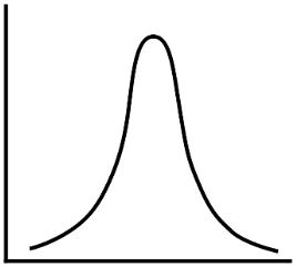
The normal distribution is also known as the Gaussian distribution. Examples of normally distributed variables include a population’s height and birth weight. Plotting a normally distributed variable using the charts above will give a familiar symmetrical, bell-shaped curve.

The normal distribution is specified by its mean and standard deviation. Other characteristics of note of normally distributed variables include:

• 68% of observations fall within one standard deviation of the mean
• 95% of observations fall within two standard deviations of the mean
• 99.7% of observations fall within three standard deviations of the mean

Non-normal distribution

There are continuous variables that do not follow the normal distribution. Examples may include household incomes and annual household expenditures.

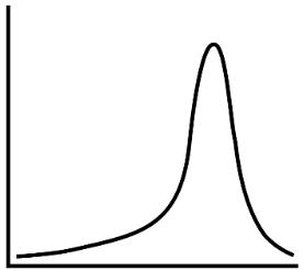
Non-normal distribution can be left-skewed (also called negatively skewed) or right-skewed (also called positively-skewed). (See images below)

Transformation of variable

Some statistical analysis can only be performed if the variables are normally distributed. Particular statistical methods can be applied to variables that are not normally distributed. An alternative approach towards analysing non-normal data is to transform the data by applying a simple function such as square root (√𝑥 ), log, or reciprocal ( 1/𝑥 ). By doing so, the data may approximate the bell-shaped curve of a normal distribution.

Binomial distribution

Categorical variables with two mutually exclusive outcomes (male or female, disease or no disease, heads or tails) have a binomial distribution. Binomial distribution describes the probability distribution of all possible outcomes (i.e. probability of obtaining five heads in a row) for a sequence of independent observations (i.e. five coin tosses).

Normal approximation of the binomial

Binomial distribution may appear different to a normal distribution when the number of observations is small. As the number of observations increases, the binomial distribution will approximate a normal distribution.

Poisson distribution

Poisson distribution also describes categorical variables. Poisson distribution describes the number of rare events occurring over a period, such as the number of cases of haematological malignancies in a paediatric population.

References

Distributions in Medical Statistics. (2017, November 18). PathBliss. https://pathbliss.com/index.php/2017/11/18/distributions-medical-statistics/ 

Describing data

Summary

A dataset can be summarised by describing its central tendency and variability.

Measures of central tendency

There are three types of measures of central tendency – mean, median, and mode.

Mean is the average of all of the data. It is obtained by adding all the values and dividing the observations. 

Where ∑ 𝑥=sum of all values, n=number of observations

The median is the middle point of all observations. The median is where half of the observations lie below and the other half lie above. 

Mode is the most commonly recorded observation. 

The central tendency is best described using the mean for normally distributed data. Interestingly, for normally distributed data, as data is spread equally on both sides of the mean, mean = median = mode.

The central tendency is best described using the median for non-normally distributed data, as outliers do not influence it. Other characteristics of measures of central tendencies in non-normally distributed data include:

• Distribution with positive skew: mode < median < mean 
• Distribution with negative skew: mean < median < mode

Measures of variability

Measures of variability describe the spread of observations. The type of measures of variability that are used depends on the data distribution.

The simplest way of describing the spread of data is by its range. The range of data states the lowest (min) and highest (max) data points. However, it provides no other information regarding the data’s distribution.

When data is normally distributed, data is symmetrically spread around the mean. Variance and standard deviation are used to describe variability.

When the data is not normally distributed, it is better to use the interquartile range. Interquartile range is the difference between observations at the 25th percentile (a.k.a. first quartile) and 75th percentile (a.k.a. third quartile).

When we repeatedly sample a population randomly, we obtain different datasets using different means. How do we measure the variability of these means? We use the standard error of the mean.

References

Frost, J. (2018a, February 12). Measures of Central Tendency: Mean, Median, and Mode. Statistics By Jim. http://statisticsbyjim.com/basics/measures-central-tendency-mean-median-mode/ 

Frost, J. (2018b, March 2). Measures of Variability: Range, Interquartile Range, Variance, and Standard Deviation. Statistics By Jim. http://statisticsbyjim.com/basics/variability-range-interquartile-variance-standard-deviation/

Frost, J. (2021, May 24). Standard Error of the Mean (SEM). Statistics By Jim. https://statisticsbyjim.com/hypothesis-testing/standard-error-mean/