14th February 2024

Normal vs. non-normal distribution

The shape of the distribution of a continuous variable can be easily determined by plotting either of the following:

• Histogram
• Frequency distribution curve
• Probability distribution curve

Normal distribution

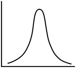
The normal distribution is also known as the Gaussian distribution. Examples of normally distributed variables include a population’s height and birth weight. Plotting a normally distributed variable using the charts above will give a familiar symmetrical, bell-shaped curve.

The normal distribution is specified by its mean and standard deviation. Other characteristics of note of normally distributed variables include:

• 68% of observations fall within one standard deviation of the mean
• 95% of observations fall within two standard deviations of the mean
• 99.7% of observations fall within three standard deviations of the mean

Non-normal distribution

There are continuous variables that do not follow the normal distribution. Examples may include household incomes and annual household expenditures.

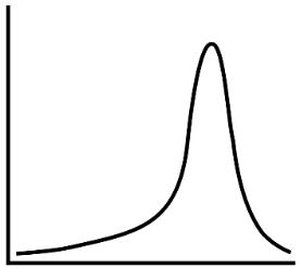
Non-normal distribution can be left-skewed (also called negatively skewed) or right-skewed (also called positively-skewed). (See images below)

Transformation of variable

Some statistical analysis can only be performed if the variables are normally distributed. Particular statistical methods can be applied to variables that are not normally distributed. An alternative approach towards analysing non-normal data is to transform the data by applying a simple function such as square root (√𝑥 ), log, or reciprocal ( 1/𝑥 ). By doing so, the data may approximate the bell-shaped curve of a normal distribution.